Analysis in Practice Part 2 - Tidy

A Small Example

Typically, when we get a dataset, we’ll see it as a series of columns (variables) with values across many rows (each an observation). This format - the wide format - is certainly amenable for human parsing, and also implies a relationship between a single observation across multiple variables.

What do I mean by this? Let’s take a look at a quick example in code of what we might get in wide format.

library(tidyverse)

wide_data <- tribble(
    ~id, ~height, ~width,
    "A",      10,     20,
    "B",      5,      11,
    "C",      7,      12
)

Note here how I’m using the tibble package tribble function to specify the data object (compared to a regular data frame). So you can see we have two variables - height and width - measured for three objects with id’s A, B, and C.

But what if instead of this wide format, we turn it into a long format? In other words, we can gather the values and make the following..

long_data <- wide_data %>%
    gather(variable, value, -id)

long_data

## # A tibble: 6 x 3
##      id variable value
##   <chr>    <chr> <dbl>
## 1     A   height    10
## 2     B   height     5
## 3     C   height     7
## 4     A    width    20
## 5     B    width    11
## 6     C    width    12

While this long format is not as easily readable for humans, it is much more readable for our tidyverse tools, such as ggplot2 for visualization, and dplyr for doing things like summaries of different variables. Let’s try the latter, and doing a summary here of height and width across our observations, A through C.

summary <- long_data %>%
    group_by(variable) %>%
    summarise(average = mean(value)) %>%
    mutate(average = round(average, digits = 2))

summary

## # A tibble: 2 x 2
##   variable average
##      <chr>   <dbl>
## 1   height    7.33
## 2    width   14.33

Here, the function names say it all: I group based on the measurement being taken, and then do a summary (in this case, an average) for each of those groups - height and width. Then the final mutate step just takes the newly created column, average, and round it down to two digits.

This is a pretty trivial example, but when you have lots of data this transformation from wide to long is extremely useful. So, to make a long story short: wide data is great for humans, and long data is great for modern R idioms of programming in the tidyverse.

Back to Our NFL QB Data

Let’s go back to our dataset from following the first post, and refresh ourselves on what it looks like:

glimpse(raw) ## Invisibly loaded/cleaned data 

## Observations: 12,556
## Variables: 13
## $ qb         <chr> "Matt Ryan", "Jameis Winston", "Mike Glennon", "Mat...
## $ att        <int> 34, 37, 11, 36, 40, 47, 36, 27, 2, 28, 1, 41, 33, 2...
## $ cmp        <int> 25, 23, 10, 23, 31, 27, 22, 16, 2, 17, 0, 22, 20, 2...
## $ yds        <dbl> 344, 261, 75, 219, 273, 364, 257, 194, 19, 149, 0, ...
## $ ypa        <dbl> 10.1, 7.1, 6.8, 6.1, 6.8, 7.7, 7.1, 7.2, 9.5, 5.3, ...
## $ td         <int> 4, 3, 1, 2, 1, 0, 4, 1, 0, 1, 0, 2, 1, 3, 0, 1, 1, ...
## $ int        <int> 0, 0, 0, 1, 0, 2, 2, 2, 0, 0, 0, 1, 0, 0, 0, 0, 1, ...
## $ lg         <chr> "32t", "28", "13", "28t", "32", "58", "46", "27", "...
## $ sack       <dbl> 2, 2, 0, 1, 2, 2, 1, 3, 0, 1, 0, 2, 2, 0, 0, 4, 2, ...
## $ loss       <dbl> 19, 10, 0, 5, 14, 17, 9, 22, 0, 12, 0, 8, 18, 0, 0,...
## $ rate       <dbl> 144.7, 110.3, 125.4, 87.6, 103.4, 64.5, 96.6, 62.9,...
## $ GamePoints <int> 43, 28, 28, 22, 16, 23, 28, 23, 23, 27, 27, 14, 19,...
## $ year       <int> 2016, 2016, 2016, 2016, 2016, 2016, 2016, 2016, 201...

A Quick Inspection and Debugging

So we can see that we have a bunch of variables for each quarterback in this wide format. Let’s turn it into the long format similar to above.

dat <- raw %>%
    gather(variable, value, -qb)
dat

## # A tibble: 150,672 x 3
##                  qb variable value
##               <chr>    <chr> <chr>
##  1        Matt Ryan      att    34
##  2   Jameis Winston      att    37
##  3     Mike Glennon      att    11
##  4 Matthew Stafford      att    36
##  5     Sam Bradford      att    40
##  6     Carson Wentz      att    47
##  7      Eli Manning      att    36
##  8 Ryan Fitzpatrick      att    27
##  9      Bryce Petty      att     2
## 10   Ryan Tannehill      att    28
## # ... with 150,662 more rows

Odd, we see that the value column is also a character! That’s not good. Let’s look at what’s causing that by trying to convert the value column to numeric, and seeing where it fails:

tmp <- dat %>%
    mutate(value = as.numeric(value))

## Warning in evalq(as.numeric(c("34", "37", "11", "36", "40", "47", "36", :
## NAs introduced by coercion

## Filter on NA values where numeric conversion fails
## Then take unique values and print first 5
dat %>%
    filter(tmp$value %>% is.na) %>%
    select(value) %>% unique %>%
    print(n = 5)

## # A tibble: 98 x 1
##   value
##   <chr>
## 1  <NA>
## 2   32t
## 3   28t
## 4   95t
## 5   65t
## # ... with 93 more rows

Hmm, so seems we have trailing ‘t’ letters in some of the values (associated with the longest throw metric). We can clip these trailing t’s using the stringr library and then do the conversion again.

.clip_t <- function(x) {
    stringr::str_replace(x, "t", "") %>%
        as.numeric %>%
            return
}

dat <- dat %>%
    mutate(value = map_dbl(value, .clip_t))

Simple Summaries

Great, so we have a long format - what can we do? Let’s again to some simple summaries, calculating the mean and standard deviations for each metric.

dat %>%
    group_by(variable) %>%
    summarise(avg = mean(value, na.rm = TRUE),
              sd = sd(value, na.rm = TRUE)) %>%
    mutate_at(vars(-variable), round, digits = 2)

## # A tibble: 12 x 3
##      variable     avg     sd
##         <chr>   <dbl>  <dbl>
##  1        att   26.87  13.62
##  2        cmp   16.12   8.81
##  3 GamePoints   21.42  10.67
##  4        int    0.80   0.97
##  5         lg   33.36  18.32
##  6       loss   11.97  11.96
##  7       rate   80.22  32.07
##  8       sack    1.86   1.70
##  9         td    1.12   1.12
## 10        yds  186.23 105.90
## 11       year 2005.94   6.12
## 12        ypa    6.88   4.20

This last step, the mutate_at, simply looks at what variables (via vars), aka columns, are present, and then applies a function (in this case, round, which takes in additional comma separated arguments (I want to round here to two digits). The vars helper function is used to provide users with the ability to use bare column names (aka no quotes) when selecting columns to mutate (similar to how the select function works by default).

An Initial Exploration with ggplot2

So great! We got some simple summaries here. But can’t we get something similar by just using the summary or apply functions? Yes, but this code is much easier to read, and then gives us the ability to do the cool bit: (gg)plotting! While a regular plot would work fine with us specifying our own columns, and is good for quick inspections, for more fanciful plots, ggplot is, as they say, bae.

To round out this post, let’s do a series of histograms for each metric.

dat %>%
    ## Specify common x-axis
    ggplot(aes(x = value)) +
    ## Create new plots for each metric
    facet_wrap(~ variable, scales = "free") +
    ## Plot histograms on each individual facet
    geom_histogram(bins = 30, colour = "white", fill = "black") +
    ## Plot Aesthetics
    labs(x = "", y = "Count") +
    cowplot::theme_cowplot(font_size = 10) +    
    theme(axis.text.x = element_text(angle = 30, hjust = 1))

## Warning: Removed 85 rows containing non-finite values (stat_bin).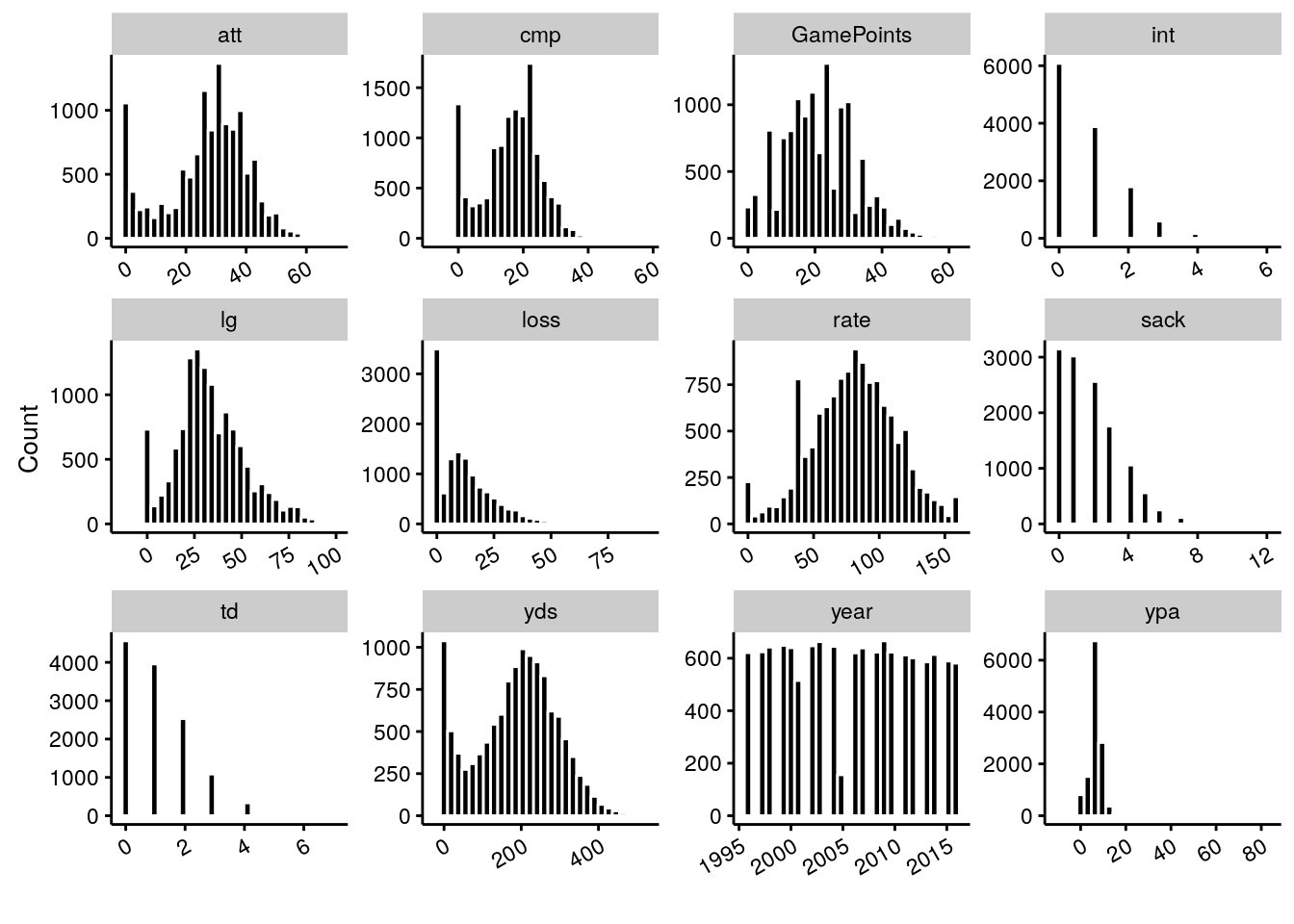

Much prettier, and much shorter than any base code. Some interesting questions to think about:

• There’s a fair number of values stacked at the 0-5 range for completions, and similarly 0-50 yard range for yards. Are these different types of QB’s (backups? wildcat plays?), and how might we remove them from consideration in estimating a QB’s efficacy?
• Which values are correlated? For example, are yards correlated with completions? Are interceptions correlated with attempts?
• How might we start to rate QBs?

So the takeaway from this post is to think about we can make data tidy, from wide to long formatting, to make it easier for us to do cool things in the tidyverse such as plotting and statistical transformations. While these were fairly toy-level examples, this tidy format will be much more useful later on. And bonus: this also helps us with doing some data debugging, as we saw here!

Of course, huge thanks to Hadley Wickham for his writing on the topic, much more eloquent than mine in explaining the concept and its many uses - check out the paper here, which ostensibly has been a driving force in the tidyverse philosophy.