One of the advantages of using Bioconductor packages is that they utilize common data infrastructures which makes analyses interoperable across various packages. Furthermore, much engineering effort is put into making this infrastructure robust and scalable. Here, we describe the SingleCellExperiment object (or sce in shorthand) in detail to describe how it is constructed, utilized in downstream analysis, and how it stores various types of primary data and metadata.
Prerequisites
The Bioconductor package SingleCellExperiment provides the SingleCellExperiment class for usage. While the package is implicitly installed and loaded when using any package that depends on the sce class, it can be explicitly installed (and loaded) as follows:
BiocManager::install('SingleCellExperiment')
Additionally, we use some functions from the scater and scran packages, as well as the CRAN package uwot (which conveniently can also be installed through BiocManager). These functions will be accessed through the <package>::<function> convention as needed.
BiocManager::install(c('scater', 'scran', 'uwot'))
For this session, all we will need loaded is the SingleCellExperiment package:
library(SingleCellExperiment)
The Essentials of sce
Primary Data: The assays Slot
The SingleCellExperiment (sce) object is the basis of single-cell analytical applications based in Bioconductor. The sce object is an S4 object, which in essence provides a more formalized approach towards construction and accession of data compared to other methods available in R. The utility of S4 comes from validity checks that ensure that safe data manipulation, and most important for our discussion, from its extensibility through slots.
If we imagine the sce object to be a ship, the slots of sce can be thought of as individual cargo boxes - each exists as a separate entity within the sce object. Furthermore, each slot contains data that arrives in its own format. To extend the metaphor, we can imagine that different variations of cargo boxes are required for fruits versus bricks. In the case of sce, certain slots expect numeric matrices, whereas others may expect data frames.
To construct a rudimentary sce object, all we need is a single slot:
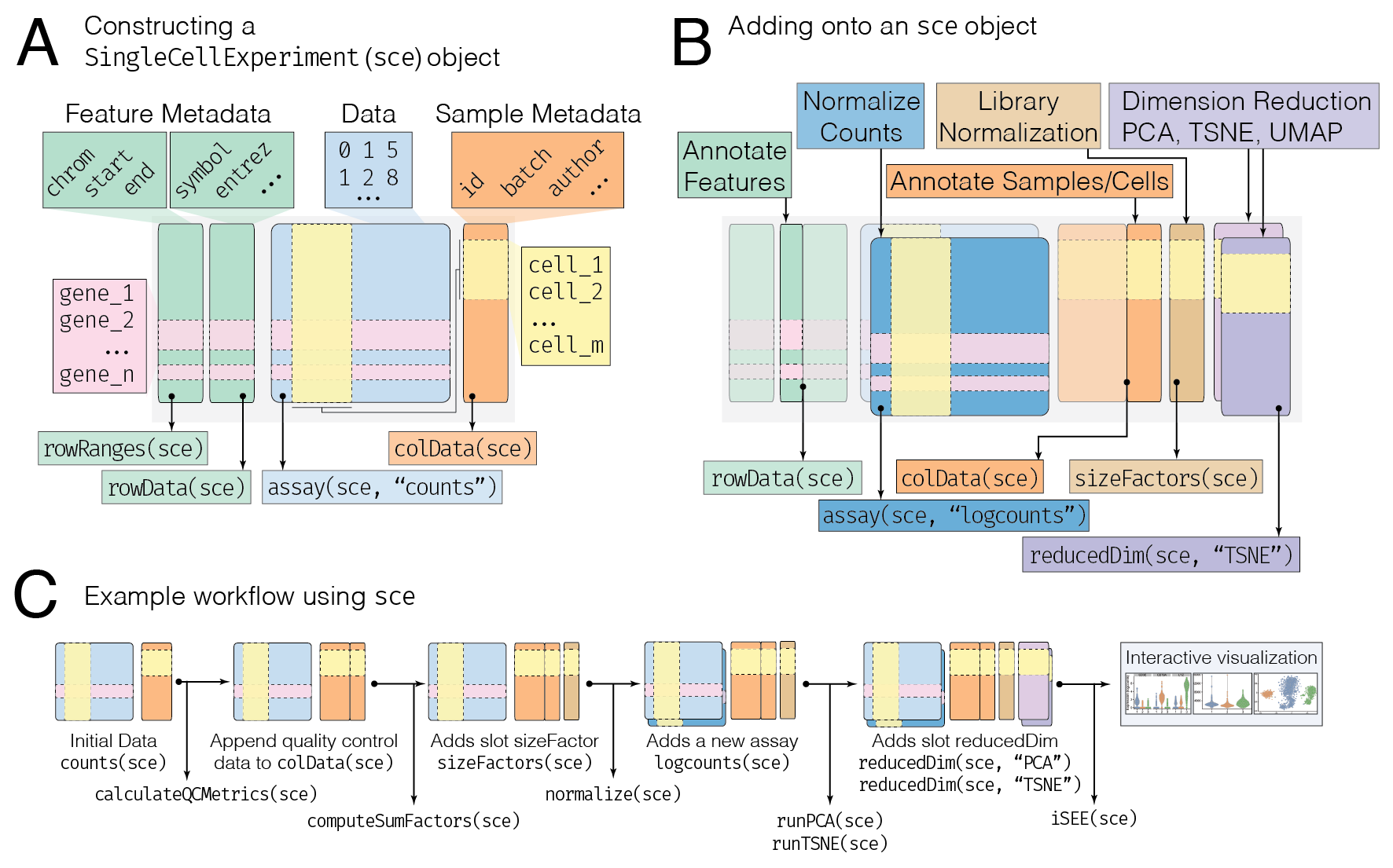
assays slot: contains primary data such as counts in list, where each entry of the list is in a matrix format, where rows correspond to features (genes) and columns correspond to samples (cells) (Figure 1A, blue box)
Let’s start simple by generating three cells worth of count data across ten genes.
counts_matrix <- data.frame(cell_1 = rpois(10, 10),
                    cell_2 = rpois(10, 10),
                    cell_3 = rpois(10, 30))
rownames(counts_matrix) <- paste0("gene_", 1:10)
counts_matrix <- as.matrix(counts_matrix) # must be a matrix object!
From this, we can now construct our first SingleCellExperiment object, using the defined constructor, SingleCellExperiment(). Note that we provide our data as a named list, and each entry of the list is a matrix. Here, we name the counts_matrix entry as simply counts within the list.
sce <- SingleCellExperiment(assays = list(counts = counts_matrix))
To inspect the object, we can simply type sce into the console to see some pertinent information, which will display an overview of the various slots available to us (which may or may not have any data).
sce
## class: SingleCellExperiment
## dim: 10 3
## metadata(0):
## assays(1): counts
## rownames(10): gene_1 gene_2 ... gene_9 gene_10
## rowData names(0):
## colnames(3): cell_1 cell_2 cell_3
## colData names(0):
## reducedDimNames(0):
## spikeNames(0):
To access the count data we just supplied, we can do any one of the following:
assay(sce, "counts") - this is the most general method, where we can supply the name of the assay as the second argument.counts(sce) - this is the same as the above, but only works for assays with the special name "counts".
counts(sce)
##         cell_1 cell_2 cell_3
## gene_1       5      5     29
## gene_2       7     11     41
## gene_3      11     11     40
## gene_4      16      3     31
## gene_5      14      7     29
## gene_6      10     12     29
## gene_7       7     12     23
## gene_8      11      5     29
## gene_9      13      7     20
## gene_10     12      7     24
## assay(sce, "counts") ## same as above in this special case
Extending the assays Slot
What makes the assay slot especially powerful is that it can hold multiple representations of the primary data. This is especially useful for storing a normalized version of the data. We can do just that as shown below, using the scran and scater packages to compute a log-count normalized representation of the initial primary data.
Note that here, we overwrite our previous sce upon reassigning the results to sce - this is because these functions return a SingleCellExperiment object. Some functions - especially those outside of single-cell oriented Bioconductor packages - do not, in which case you will need to append your results to the sce object (see below).
sce <- scran::computeSumFactors(sce)
sce <- scater::normalize(sce)
Viewing the object again, we see that these functions added some new entries:
sce
## class: SingleCellExperiment
## dim: 10 3
## metadata(1): log.exprs.offset
## assays(2): counts logcounts
## rownames(10): gene_1 gene_2 ... gene_9 gene_10
## rowData names(0):
## colnames(3): cell_1 cell_2 cell_3
## colData names(0):
## reducedDimNames(0):
## spikeNames(0):
Specifically, we see that the assays slot has grown to be comprised of two entries: counts (our initial data) and logcounts (the normalized data). Similar to counts, the logcounts name is a special name which lets us access it simply by typing logcounts(sce), although the longhand version works just as well.
logcounts(sce)
##         cell_1 cell_2 cell_3
## gene_1    3.10   3.46   4.07
## gene_2    3.53   4.53   4.54
## gene_3    4.14   4.53   4.51
## gene_4    4.66   2.81   4.16
## gene_5    4.47   3.91   4.07
## gene_6    4.01   4.65   4.07
## gene_7    3.53   4.65   3.75
## gene_8    4.14   3.46   4.07
## gene_9    4.37   3.91   3.57
## gene_10   4.26   3.91   3.81
## assay(sce, "logcounts") ## same as above
Notice that the data before had a severe discrepancy in counts between cells 1/2 versus 3, and that normalization has ameliorated this difference.
To look at all the available assays within sce, we can type:
assays(sce)
## List of length 2
## names(2): counts logcounts
While the functions above demonstrate automatic addition of assays to our sce object, there may be cases where we want to perform our own calculations and save the result into the assays slot. In particular, this is important for using functions that do not return your SingleCellExperiment object.
Let’s append a new version of the data that has been offset by +100.
counts_100 <- assay(sce, "counts") + 100
assay(sce, "counts_100") <- counts_100 # assign a new entry to assays slot
Then we can use the accessor assays() (notice this is plural!) to see all our entries into the assay slot that we have made so far. Note that to see the names of all the assays, we use the plural assays() accessor, and to retrieve a single assay entry (as a matrix) we use the singular assay() accessor, providing the name of the assay we wish to retrieve as above.
assays(sce)
## List of length 3
## names(3): counts logcounts counts_100
These entries are also seen on the default view of sce:
sce
## class: SingleCellExperiment
## dim: 10 3
## metadata(1): log.exprs.offset
## assays(3): counts logcounts counts_100
## rownames(10): gene_1 gene_2 ... gene_9 gene_10
## rowData names(0):
## colnames(3): cell_1 cell_2 cell_3
## colData names(0):
## reducedDimNames(0):
## spikeNames(0):
This sort of extension of the assays slot is represented graphically in Figure 1B (dark blue box), showing the addition of the logcounts matrix into the assays slot.
In a similar manner, many of the slots of sce are extendable through assignment as shown above, thus allowing for myriad custom functionality as needed for interoperability with functions outside of single-cell oriented Bioconductor packages.
Column (Meta)Data: colData Slot
To further annotate our sce object, one of the first and most useful pieces of information is adding on metadata that describes the columns of our primary data, e.g. describing the samples or cells of our experiment. This data is entered into the colData slot:
colData slot: metadata that describes that samples (cells) provided as a data.frame or (DataFrame if appending), where rows correspond to cells, and columns correspond to the sample (cells) metadata features (e.g. id, batch, author, etc.) (Figure 1A, orange box).
So, let’s come up with some metadata for the cells, starting with a batch variable, where cells 1 and 2 are in batch 1, and cell 3 is from batch 2.
cell_metadata <- data.frame(batch = c(1, 1, 2))
rownames(cell_metadata) <- paste0("cell_", 1:3)
Now, we can take two approaches - either append the cell_metadata to our existing sce, or start from scratch via the SingleCellExperiment() constructor and provide it from the get go. We’ll start from scratch for now, but will also show how to append the data as well:
## From scratch:
sce <- SingleCellExperiment(assays = list(counts = counts_matrix),
                           colData = cell_metadata)

## Appending to existing object (requires DataFrame() coercion)
## colData(sce) <- DataFrame(cell_metadata)
Similar to assays, we can see our colData is now populated from the default view of sce:
sce
## class: SingleCellExperiment
## dim: 10 3
## metadata(0):
## assays(1): counts
## rownames(10): gene_1 gene_2 ... gene_9 gene_10
## rowData names(0):
## colnames(3): cell_1 cell_2 cell_3
## colData names(1): batch
## reducedDimNames(0):
## spikeNames(0):
And furthermore access our column (meta)data with the accessor, colData():
colData(sce)
## DataFrame with 3 rows and 1 column
##            batch
##        <numeric>
## cell_1         1
## cell_2         1
## cell_3         2
Finally, some packages automatically add to the colData slot, for example, the scater package features a function, calculateQCMetrics(), which appends a lot of quality control data. Here we show the first five columns of colData(sce) with the quality control metrics appended to it.
sce <- scater::calculateQCMetrics(sce)
colData(sce)[, 1:5]
## DataFrame with 3 rows and 5 columns
##            batch is_cell_control total_features_by_counts
##        <numeric>       <logical>                <integer>
## cell_1         1           FALSE                       10
## cell_2         1           FALSE                       10
## cell_3         2           FALSE                       10
##        log10_total_features_by_counts total_counts
##                             <numeric>    <integer>
## cell_1               1.04139268515823          106
## cell_2               1.04139268515823           80
## cell_3               1.04139268515823          295
Using colData for Subsetting
A common operation with colData is its use in subsetting. One simple way to access colData is through the use of the $ operator, which is a shortcut for accessing a variable within the colData slot:
sce$batch
## [1] 1 1 2
## colData(sce)$batch # same as above
If we only wanted cells within batch 1, we could subset our sce object as follows (remember, we subset on the columns in this case because we are filtering by cells/samples here).
sce[, sce$batch == 1]
## class: SingleCellExperiment
## dim: 10 2
## metadata(0):
## assays(1): counts
## rownames(10): gene_1 gene_2 ... gene_9 gene_10
## rowData names(7): is_feature_control mean_counts ... total_counts
##   log10_total_counts
## colnames(2): cell_1 cell_2
## colData names(10): batch is_cell_control ...
##   pct_counts_in_top_200_features pct_counts_in_top_500_features
## reducedDimNames(0):
## spikeNames(0):
Size Factors Slot: sizeFactors
Briefly, we already encountered this via the scran::computeSumFactors(sce) call, which adds a sizeFactors slot:
sizeFactors slot: contains information in a numeric vector regarding the sample/cell normalization factors used to produce a normalize data representation (Figure 1B, brown box)
sce <- scran::computeSumFactors(sce)
sce <- scater::normalize(sce)
sizeFactors(sce)
## [1] 0.661 0.499 1.840
The reducedDims Slot
The reducedDims slot is a new addition which is specially designed to store the reduced dimensionality representations of primary data, such as PCA, tSNE, UMAP, and others.
reducedDims slot: contains a list of numeric matrix entries which describe dimensionality reduced representations of the primary data, such that rows represent the columns of the primary data (aka the samples/cells), and columns represent the dimensions
Most importantly, just like the assays slot, the reducedDims slot can hold a list of many entries. So, it can hold a PCA, TSNE, and UMAP representation of a given dataset all within the reducedDims slot.
In our example, we can calculate a PCA representation of our data as follows using the scater package function runPCA(). We see that the sce now shows a new reducedDim and that the accessor reducedDim() produces the results of running PCA on the normalized data from logcounts(sce).
sce <- scater::runPCA(sce)
reducedDim(sce, "PCA")
##           PC1    PC2
## cell_1 -2.991 -0.516
## cell_2  2.218 -1.345
## cell_3  0.773  1.861
## attr(,"percentVar")
## [1] 0.723 0.277
From this, we can also calculate a tSNE representation using the scater package function runTSNE(), and see that it can be seen both in the default view of sce and via accession:
sce <- scater::runTSNE(sce, perplexity = 0.1)
## Perplexity should be lower than K!
reducedDim(sce, "TSNE")
##         [,1]  [,2]
## cell_1  3331 -4621
## cell_2 -5666  -571
## cell_3  2335  5192
We can view the names of all our entries in the reducedDims slot via the accessor, reducedDims() (notice that this is plural, and thus not the same as reducedDim():
reducedDims(sce)
## List of length 2
## names(2): PCA TSNE
Now, say we have a different dimensionality reduction approach which has not yet been implemented with SingleCellExperiment objects in mind. For example, let’s say we want to try the umap() function as implemented in the uwot package (which is a much faster version of the default umap implementation currently in scater).
Similar to how we extended the assays slot with our own custom entry of counts_100, we can do similarly for the reducedDims slot:
u <- uwot::umap(t(logcounts(sce)), n_neighbors = 2)
reducedDim(sce, "UMAP_uwot") <- u

reducedDim(sce, "UMAP_uwot")
##          [,1]   [,2]
## cell_1 -0.269  0.581
## cell_2  0.569 -0.348
## cell_3 -0.300 -0.233
## attr(,"scaled:center")
## [1] -11.88  -2.51
And we can also see its entry when we look at the reducedDims() accessor output:
reducedDims(sce)
## List of length 3
## names(3): PCA TSNE UMAP_uwot